Inconsistent Maximum Likelihood Estimation: An “Ordinary” Example
2008-08-09 at 6:24 pm 44 comments
The widespread use of the Maximum Likelihood Estimate (MLE) is partly based on an intuition that the value of the model parameter that best explains the observed data must be the best estimate, and partly on the fact that for a wide class of models the MLE has good asymptotic properties. These properties include “consistency” — that as the amount of data increases, the estimate will, with higher and higher probability, become closer and closer to the true value — and, moreover, that the MLE converges as quickly to this true value as any other estimator. These asymptotic properties might be seen as validating the intuition that the MLE must be good, except that these good properties of the MLE do not hold for some models.
This is well known, but the common examples where the MLE is inconsistent aren’t too satisfying. Some involve models where the number of parameters increases with the number of data points, which I think is cheating, since these ought to be seen as “latent variables”, not parameters. Others involve singular probability densities, or cases where the MLE is at infinity or at the boundary of the parameter space. Normal (Gaussian) mixture models fall in this category — the likelihood becomes infinite as the variance of one of the mixture components goes to zero, while the mean is set to one of the data points. One might think that such examples are “pathological”, and do not really invalidate the intuition behind the MLE.
Here, I’ll present a simple “ordinary” model where the MLE is inconsistent. The probability density defined by this model is free of singularities (or any other pathologies), for any value of the parameter. The MLE is always well defined (apart from ties, which occur with probability zero), and the MLE is always in the interior of the parameter space. Moreover, the problem is one-dimensional, allowing easy visualization.
The data consists of i.i.d. real values x1, x2, …, xn. The model has one positive real parameter, t. The distribution of a data point is an equal mixture of the standard normal and a normal distribution with mean t and standard deviation exp(-1/t^2):

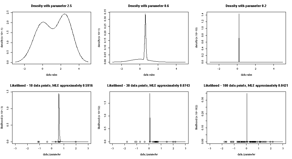
Using this R program, I produced some plots of densities and likelihood functions derived from this model.
Looking at the top left plot, the probability density function when t=2.5, you can see two modes near 0 and t. As t decreases to 0.6, and then 0.2, the mode at t moves left and gets narrower. A narrower mode has higher probability density at its peak. When t=0.2, the peak density of the mode at t is about 1010 times higher than the peak density of the mode at 0, which is invisible at the scale of the plot (the scale is noted in the left-side caption).
The bottom plots are of likelihood functions given data generated from the model with t=0.6. I generated 100 points, and used the first 10, the first 30, and all 100 for the three plots. With 10 data points, the value that maximizes the likelihood (0.5916) is close to the true parameter value (0.6). But as the number of data points increases, the MLE moves away from the true value, getting closer and closer to zero. The value of the likelihood at the MLE also gets bigger, reaching about 0.3×10162 when 100 data points are used.
This plot shows the likelihood function with 30 data points with the vertical scale changed to show detail other than the peak. A local maximum of the likelihood around the true value of 0.6 can now be seen. It is completely dominated by the maximum at 0.0743, which is about a factor of 1052 higher.
Why does this happen? First, note that regardless of the true value of t, the density in the vicinity of zero will be non-singular, so the probability that a data point will land in the interval (0,c) will be proportional to c when c is small. In a data set of n points, we can therefore expect the smallest positive data point, call it x0, to have a magnitude of about k/n, for some constant k. Now, consider the value of the log likelihood function at t=x0 versus its value at the true value of t. When t=x0, the log probability density for x0 will be approximately

In comparison, the density of x0 when t is not close to x0 will be approximately half its density under the N(0,1) distribution, which will approach a constant as n increases (and x0 goes to zero). The density under t=x0 for data points other than x0 will approach a constant as n increases and t goes to zero. On average, the true value of t (or values near the true value) will produce a higher value for the density of such points, but the difference in log densities will approach a constant. The end result is that the contribution to the log likelihood of data points other than x0 will be greater for the true value of t than for t=x0 by an amount that grows in proportion to n, while the contribution to the log likelihood of the point x0 will be greater for t=x0 than for the true value of t by an amount that grows in proportion to n2. As n increases, the n2 contribution will dominate, so the MLE will be close to zero rather than being close to the true value of the parameter. (Note, however, that the MLE will usually not be exactly equal to x0, though when n is large it will usually be nearby. The argument above just shows that a value of t near x0 will have higher likelihood than a value near the true value of t.)
So what does this say about the Maximum Likelihood intuition — that the best estimate is the parameter value that best explains the data? It illustrates the Bayesian critique of this intuition, which is that using the MLE ignores the volume of the parameter space where the data is fit well. When n is large, only a tiny region around x0 fits the data better than the true value of the parameter. In a posterior distribution (based on some prior), the smallness of this region will cancel the large height of the peak, with the result that the posterior probability that t is near x0 will usually not be large.
Entry filed under: Statistics, Statistics - Technical.
44 Comments Add your own
Leave a comment
Trackback this post | Subscribe to the comments via RSS Feed

1. Kevin Canini | 2008-08-20 at 7:55 am
This is an interesting post. I didn’t realize that cases where the MLE is inconsistent could be so simple. Anyway, I’m confused about the last paragraph. How would taking the MAP value of the parameter fix this pathology? For example, if an improper uniform prior (or a very wide normal distribution) were used, I don’t see how the MAP estimate would differ much from the MLE estimate. And isn’t the MLE analog of the “posterior probability that t is near x_0” (i.e., the integral of the likelihood function around x_0) going to be small anyway, since the tall spike is so narrow?
2. radfordneal | 2008-08-20 at 10:56 am
You’re right that the MAP estimate would be much the same as the MLE. But MAP estimates aren’t Bayesian – they are better referred to as “maximum penalized likelihood” estimates. If you were to look at an estimate that pays attention to the whole posterior distribution, like the posterior median or the posterior mean, you’d get something quite different from the MLE.
In an non-Bayesian framework, integrals of the likelihood function are not done. So there’s no concept of integrating the likelihood over the neighborhood of the MLE. That would be a Bayesian method with the prior happening to be uniform.
The big difference between Bayesian and non-Bayesian methods is that Bayesian methods integrate over the parameter space, and non-Bayesian methods don’t. To integrate, one needs a base measure – ie, a prior distribution – so Bayesian methods inevitably involve a prior, but from this (somewhat mathematical) point of view, the prior isn’t the central issue.
3. Corey | 2012-06-11 at 12:37 am
“In an non-Bayesian framework, integrals of the likelihood function are not done.”
Just dropped by to refresh my memory of this model. In point of fact Thomas Severini had a paper on the subject at the time the above comment was written. There’s been another one since.
4. Radford Neal | 2012-06-11 at 9:32 am
From a quick glance at the abstracts, the methods in those papers seem to be “semi-Bayesian”. They have a part of a prior, for nuisance parameters given a parameter of interest, allowing them to integrate over the nuisance parameter, but the results are viewed in non-Bayesian terms.
Integration is always with respect ot some measure, which one might call a “prior”, and if you think having a “prior” means you’re “Bayesian”, then my statement is true. You might not think that, of course, but my point was really that you have to add something like a prior to the MLE framework before you can sensibly talk about integration over points near the MLE, as in the first comment.
5. Bill Jefferys | 2008-08-20 at 9:02 pm
Radford, this would be a whole lot easier to visualize if you would rescale the pix so that they were all on the same horizontal scale. As it is, it’s not easy to see the effect you rightly point out. Since the likelihood isn’t a density, the vertical scale can be set any way you wish.
I would think that roughly (-2,+3) would work well.
6. Corey | 2008-08-20 at 10:08 pm
Which of the regularity conditions that one normally handwaves away is being violated here?
7. radfordneal | 2008-08-20 at 10:35 pm
Bill,
I maybe didn’t explain the plots well enough. The top row of plots are of the data density for various values of the parameter. There’s no actual data involved in these. They all have a horizontal range (for possible data points) of about (-3,5). But note that the vertical scale changes drastically (see the multiplication factor in the axis label). These plots are meant just to demonstrate how as the parameter gets closer to zero, a mode near the parameter value moves closer to zero too, and gets narrower and narrower.
The lower plots are of the data and the corresponding likelihood function for 10, 30, and 100 points from a data set. The horizontal axis does double duty for both data values and parameter values (these are distinct, but closely related for this model). The horizontal range for all these lower plots is (-3,3), so you can compare what happens to the likelihood function (and hence the MLE) as the number of data points increases. Note that the likelihood function is plotted only for positive values, since I restricted the parameter to be positive (though the data can be negative). The horizontal range is (-3,3) for the later “zoomed in” likelihood plot too.
8. Adam | 2008-08-21 at 5:25 pm
Isn’t it possible that this is because that the discrete sample representation of the true probability density is inaccurate. It seems one needs infinite number of samples to accurately represent a continuous distribution. If we have infinite number of samples, then this infinity maybe able to cancel the infinity induced by the density concentrated at zero such that the maximal mode is still located at the true value instead of zero.
9. Radford Neal | 2008-08-21 at 6:20 pm
Adam,
The notion of consistency I’m using in this post is the usual one, which is more specifically referred to as “weak” consistency – as the amount of data increases, the estimate will, with higher and higher probability, become closer and closer to the true value. There’s another notion, called “Fisher consistency”, which is related to what you’re thinking of. It applies only when you can sensibly view the estimate as a function of the empirical distribution, in which case you can ask what happens when you apply it to the actual distribution. If it gets the right answer then, it’s Fisher consistent.
For example, consider estimating the mean of a normal distribution by the sample median. This is Fisher consistent, because the median of a normal distribution is indeed equal to its mean. (The sample median is also weakly consistent.)
Maximum likelihood estimates are always going to be Fisher consistent (assuming they’re well defined). This is related to how the Kullback-Leibler divergence between distributions is zero only for the divergence between a distribution and itself. Fisher consistency isn’t of any practical use, however, (at least for continuous distributions) since we’re always dealing with finite samples.
10. Radford Neal | 2008-08-22 at 3:38 pm
Corey asks,
Which of the regularity conditions that one normally handwaves away is being violated here?
That depends on which MLE consistency theorem one looks at, of course, but once one gets beyond theorems for models with a finite number of values for the parameters, the conditions go beyond easily-checked things like continuity. The example here has all the non-singularity and continuity one might want. (The parameter space is non-compact, but that’s true for most models used in practice.)
For example, in Theory of Statistics by Mark Schervish Theorem 7.49 plus Lemma 7.54, a crucial condition involves the expected value of the largest difference in log probability for a single data point given by the true parameter value and the log probability given by the parameter value in some region that best fits that data point. For this model, one needs to look at a region extending towards zero, and this expected value ends up as minus infinity, basically because -1/t^2 integrates to minus infinity over a region near zero. This is related to the argument in the post for why the MLE for this model won’t be consistent.
11. sv | 2008-08-23 at 11:29 pm
This is very interesting. For those of us not who don’t have any experience with the Bayesian methods, would it be possible to show the Bayesian solution as well?
12. Corey | 2008-08-24 at 2:51 pm
Thanks! Putting it that way makes it seems — well, not obvious — but in obvious agreement with one’s intuition about how MLE consistency should (fail to) work.
13. Radford Neal | 2008-08-24 at 3:00 pm
Another point regarding how this example fails to satisfy the premises of theorems about consistency of the MLE… I can’t recall seeing a theorem to this effect, but I think one could prove the MLE is consistent for a bounded parameter space (as here, if we impose an upper limit on t, which wouldn’t affect the example) provided there is an upper bound on the probability density, for any parameter value and any data point. This isn’t satisfied by this example, of course.
My intuition for why such a theorem should be possible is that under these conditions a finite discretization of the parameter space should give a good approximation to the model for all parameter values. And the MLE will be consistent if the parameter space is finite. Maybe sometime I’ll try formalizing this (if it hasn’t already been done).
14. Meng | 2008-08-24 at 8:33 pm
“finite parameter space” may be relaxed to “being bounded away from zero” in this example or similar conditions in general, I think.
15. Meng | 2008-08-24 at 9:27 pm
Re: Adam
A sample size of 30 can be large enough to well represent the true density. You may draw a histogram to see this. Actually as illustrated by Radford, it will be even worse with more samples.
“the infinity induced by the density concentrated at zero” is a (infinite) value of the likelihood function at a parameter point (close to zero). The value of the likelihood function at a parameter value equals to the product (or sum in log-scale) of the values of the density function at each data point with that parameter value. Therefore, for a given parameter value, how large the likehood function is is a combined effect from all the data points through their density function. However, if one data point has some type of dominant contribution (e.g. infinite density value), averaging over even a large number of values may not be able to remove atypical phenonimena like “infinity”.
My opinion though.
16. Radford Neal | 2008-08-24 at 9:58 pm
Meng,
In this example, parameter values just above zero are the source of the problem, but of course other values might be the problem for other models. By “finite parameter space” I meant that that there are only a finite number of possible values for the parameter (so the parameter space isn’t an interval of the real line, for instance). An approximation with a finite parameter space will be good for all values of the parameter if slight changes in parameter values don’t have huge effects. In the model of this post, that’s not true, because even though the density never becomes singlular (so there aren’t any infinite density values), it does become increasingly peaked as the parameter gets closer to zero.
17. Keith O'Rourke | 2008-08-25 at 3:07 pm
Looking at how the individual observation likelihood components combine (and contrast with each other) can be useful.
This example is interesting to me because even though we know the observations were generated with a single (common) parameter most individual observation likelihoods support .6 but a few support (different?) small values around zero – and these few out weigh the majority… so the parameter value most likley to generate this set of observations is “misleading”.
Simple modifications the the plot.lik code to get these plots are given below (on the log scale).
cheers
Keith
function (x,…)
{
grid 0 & x<3],seq(0.01,3,by=0.01)))
ll <- rep(NA,length(grid))
for (i in 1:length(grid))
{ ll[i] <- log.lik(x,grid[i])
}
mlv <- max(ll)
mle <- grid[ll==mlv][1]
max.ll <- round(mlv/log(10))
#ll <- ll – max.ll*log(10)
#lik <- exp(ll)
mlvi=(1:length(grid))[ll==mlv]
ll <- ll – ll[ll==mlv] + 2
lik <- ll
plot(c(-0,2),c(-8,max(lik) + 2),type=”n”,
xlab=”data / parameter”,
ylab=paste(“likelihood (x 10^”,max.ll,”)”,sep=””),
…)
points(x,rep(0,length(x)),lty=19)
lines(grid,lik)
title(paste(“Likelihood -“,length(x),”data points,”,
“MLE approximately”,round(mle,4)))
iol=NULL
for(k in 1:length(x)){
for(ki in 1:length(grid))
iol[ki]=log.lik(x[k],grid[ki])
lines(grid,iol – iol[mlvi] + 2/length(x),col=2)}
}
18. Radford Neal | 2008-08-25 at 9:23 pm
Keith,
I think the code got sort of destroyed in your comment by the blog software interpreting less-than and greater-than signs as HTML commands. To get a less-than through, you have to use ampersand, “lt”, semicolon. I think…
Here’s a try: < Worked?
19. Anonymous | 2008-08-26 at 11:05 am
I’ll resend when I am back at my usual computer
Occured to me this morning if one took account of observations being actually discrete rather than truly continuous and replaced the density with the integral from obs – e to obs + e the inconsistency would go away – if e was big enough?
cheers
Keith
20. Keith O'Rourke | 2008-08-26 at 11:07 am
Last comment was from me – forgot to enter email and name ;-)
Keith
21. Radford Neal | 2008-08-26 at 2:47 pm
if one took account of observations being actually discrete rather than truly continuous and replaced the density with the integral from obs – e to obs + e the inconsistency would go away – if e was big enough?
Yes. In that case, the data space would be finite (we can ignore the infinity in the big direction), and with enough data, the probability of each of these possible data values would be very well estimated. Values for the single model parameter map to distributions over these finite number of data values, in a continuous and probably one-to-one fashion, allowing the parameter to be well estimated by maximum likelihood.
However, you shouldn’t conclude that results about inconsistencies of MLEs aren’t relevant in practice, since data is always rounded. The practical effect of an inconsistent MLE is that the MLE also isn’t very good for finite amounts of data. Even if the data is rounded, so the MLE is consistent, this bad performance for finite amounts of data may remain. In a problems with higher-dimensional data, even fairly coarse rounding will still produce a huge number of possible data values, so that the finiteness may not be of any practical relevance.
22. Radford Neal | 2008-08-26 at 9:35 pm
Keith,
Here are the R program and plots produced by it that you sent by email. I haven’t absorbed the plots entirely, but it’s certainly the case that the inconsistency of the MLE is due to a few (one, typically) data points dominating.
23. Four Years Remaining » Blog Archive » Maximum Likelihood for Incomplete Data | 2008-11-27 at 2:11 pm
[…] turns out to be quite a reasonable suggestion, which leads to good estimates (although, there are some rare exceptions). Here, for example, it turns out that to estimate the mean you should simply compute the average […]
24. ekzept | 2009-07-10 at 1:32 am
Regarding “The big difference between Bayesian and non-Bayesian methods is that Bayesian methods integrate over the parameter space, and non-Bayesian methods don’t”, frequentist methods are not the only non-Bayesian method. There are also Kullback-Leibler methods, means of inference based upon divergence measures between likelihood functions. See for instance Burnham and Anderson, Wildlife Research, 2001, 28, 111–119, “KL information as a basis for strong inference in ecological studies.”
25. Oleg M. | 2009-11-17 at 2:18 pm
Did I misunderstand the example?
I tried to replicate this example, and here is my code
t <- 0.6
n <- 100
ind <- sample(c(0,1), n, replace = T) # this is 0/1/ indicator for the mixture
X <- ind*rnorm(n) + (1-ind)*rnorm(n,t,exp(-1/t^2)) # this generates X’s from Neal’s example
trange <- seq(0,1,0.0001)
loglik <- function(th){
sum(log(0.5*dnorm(X) + 0.5*dnorm(X,th,exp(-1/th^2)) ) )
}
LLt <- trange*0
for (i in 1:length(trange)){
LLt[i] <- loglik(trange[i])
}
plot(trange, LLt, type=”l”)
j <- which.max(LLt)
(mle <- trange[j])
According with this, there are *no problems whatsoever* with the MLE.
26. Radford Neal | 2009-11-18 at 2:02 am
Looking at your program, I think you haven’t misunderstood the model. However, you’ve haven’t realized how serious the numerical issues with finding the true MLE are.
You will have generated a different sample of 100 points than I used, so I can’t say for sure exactly what happened. But one possible problem is floating-point overflow / underflow. Your first grid point for t (other than 0, which you shouldn’t really have included) is 0.0001. The standard deviation for this value, which is exp(-1/0.0001^2), will underflow to zero.Another problem is that your grid isn’t fine enough. The smallest positive data point may be around 0.01. For values of t around there, the standard deviation is around exp(-1/0.01^2), which also underflows to zero, and hence is certainly much smaller than your grid spacing of 0.0001. So your grid is likely to just skip from one side of the MLE to the other without seeing any point close enough to the MLE for it to have a higher likelihood than the likelihood in the vicinity of the true parameter value.
The R program I link to just after the first equation goes to considerable lengths to avoid these numerical problems.
27. Quora | 2012-03-10 at 2:08 pm
In which situations should we use minimum MSE estimates, Unbiased estimates, and MLE estimates respectively?…
In general, if you know estimator [math]T[/math] has lower MSE than estimator [math]U[/math] for all possible values of the unknown parameters, you should choose [math]T[/math] over [math]U[/math]. (If squared error loss is not appropriate, substitute …
28. Radford Neal | 2012-03-10 at 5:00 pm
Yes, that’s known as T “dominating” U, and would seem to be a good reason not to use U, though examples like the fact that the “James-Stein estimator” for the mean of a vector in three or more dimensions dominates the simple sample mean make this less obvious than one might have thought…
29. IT | 2014-10-20 at 2:55 pm
I’m reading a comment to a paper, and the author states that sometimes, even though the estimators (found by ML or maximum quasilikelihood) may not be consistent, the test may be consistent. How and when does this happen? Do you know of some bibliography?
Click to access Testing%20for%20Regime%20Switching%20A%20Comment.pdf
30. Jose M Vidal-Sanz | 2015-03-13 at 10:31 pm
For non-smooth enough or asymmetric likelihoods, the sample size required to get good asymptotic properties can be very high. This is well known even in trivial examples, for example try to apply the CLT to the mean of (Xi)**2, for i=1,…,n. Even if Xi are i.i.d. normally distributed you will need a very large sample size n, this is why a chi-square is used and not the CLT. In a more complex estimator, such as maximum likelihood you should never expect a small sample size to get good results.
The ML estimator for the considered likelihood function is perfectly consistent and asymptotically normal (provided t>0). This is a mathematical fact. Consistence or asymptotic normality are theorems, not simulations. In this case, it is. Naturally, the second step is to obtain a bound on the error committed approximating the distribution of the estimator by a normal variable, and that is provided by the Berry-Esseen Theorem, form where you will know that a large n is required, or alternatively if your sample is small (30 or 100) at least you should use an Edgeworth Expansion approximation instead of a normal. So theory works well, but you need to be more careful.
The post shows clearly how misleading is to use simulations as a poor substitute of mathematics, and therefore it does not prove inconsistence, just that sample sizes must be larger. But to show it you need a full simulation. Run a Monte Carlo with 5.000 sample draws, and take n=10.000 and then take a look to the results. There is nothing in the model that affects consistency or asymptotic normality.
31. Radford Neal | 2015-03-14 at 9:30 am
I think you should read the post again, and think about it. It’s not an issue of a large sample size being needed. The estimate is actually more likely to be bad for a large sample size than for a small sample size. That’s because it’s inconsistent. Since it’s inconsistent, there is obviously no point in discussing asymptotic normality.
You claim that consistency of this MLE is “a mathematical fact”, demonstrated by some theorem, which you don’t quote. There are lots of theorems about consistency of the MLE. They all have premises. The conclusion only holds if the premises hold. They don’t in this case.
32. Corey | 2015-03-14 at 1:51 pm
Jose, when this example was first posted I asked about what regularity assumption was being violated to give rise to this inconsistency, and Professor Neal gave one such in comment #10 above.
33. Brad | 2017-03-29 at 9:17 pm
I’m going to go out on a limb here, but I think the issue is that the described analysis is NOT optimizing likelihood, rather point sampled likelihood density.
L(Data)=P(Data|Model). For normally distributed IID data, this likelihood represented by the product point sampled Gaussians CAN be a good approximation of un-normalized probability, but aren’t always. Here they are not, for the peaked distribution surrounding the point closest to zero (singling out that point as sigma ->0) .
As likelihood is a probability, L(D) is never >1. I believe the issue here is in a problematic estimate of likelihood, not inconsistency of the MLE.
34. Radford Neal | 2017-03-30 at 12:08 am
It’s standard to define a likelihood function using a probability density function, when the data is continuous, so it’s quite common for likelihoods to be numerically evaluated as being greater than 1. However, theoretically, a likelihood is by definition an equivalence class of functions of parameters differing only in an overall constant factor, so it doesn’t even make sense to ask if a likelihood is greater than one.
Trying to think what you might be thinking, however, my guess is that you think that all real data is discrete, not continuous, and hence all real likelihoods are based on probability mass functions, not probability density functions. There’s something to be said for this view, and it does formally eliminate the inconsistency of the MLE in this example if you assume that the data has limited precision.
However, in high-dimensional problems the finite space of possible data sets is extremely large, even assuming individual values are rounded to not-too-much precision. It may then be more enlightening to consider continuous data (even if that’s an unrealizable idealization) than to trust that the MLE is guaranteed to be consistent in finite settings, when convergence to the correct value may in practice occur extremely slowly.
35. Vitya | 2017-09-23 at 12:09 pm
Can I summarize the findings? I found that example to be even more (obviously) pathological than some mentioned in the first paragraph. What it basically says, is that if I constructed a family of probabilities with diverging probability functions with no-zero chance to hit the data point, MLE will certainly max out at a wrong distribution.
Example, my ‘family’ is a function of t: at one end (say t0) it does not include delta function. (Delta function is just an extreme, showing how absurdly narrow distributions in my/your ‘family’ could be)
Such a ‘family’ will never converge to a right original distribution because as it hits any data point, it MLE will diverge for t <0.
I do want to point out that it is a great lesson and amazing work nevertheless, I simply disagree that it is an ORDINARY example. Boy, its anything but, It includes divergent likely-hoods.
Am I getting something wrong here? It's always good to know if you are wrong, that's where we learn the most.
36. Radford Neal | 2017-09-23 at 12:34 pm
What is “ordinary” or “pathological” is a matter of opinion. But the example I give does avoid some of the obvious things that one might think might make it irrelevant to “real” problems. In particular, it is NOT the case that the likelihood is ever infinite, for any non-zero value of t, nor is it the case that the MLE will be exactly at a data point. Of course, the distributions do in some sense get a bit “extreme” for some values of t.
At the other extreme, for models in which the parameter space is a finite set, the MLE will certainly be consistent.
Looking at both of these extremes may give you more insight into what to expect from an MLE.
37. Priyanka Sinha | 2018-07-14 at 11:42 am
I believe I’m facing a similar situation, where my MLE tends to get closer and closer to (0,0), far away from it’s true value,as number of data samples go higher. Using priors in form a maximum a-posterior estimator did not help me much, as the value of the log likelihood function is a much smaller negative number (range -4000 to 0) as compared to the log of the prior (range -5 to 0), for the prior to have any significant contribution toward the objective function. However penalizing the log likelihood by multiplying it with a small fraction, so that the ranges for the likelihood and the prior will be comparable, helped a little bit. There are couple of issues now, how to justify the adhocery of this penalization/regularization approach? Is it at all the right way to go? Is there a formal way of doing this? How can I prove formally that my MLE is inconsistent?
Id appreciate any suggestions you might have to offer. I’m also not sure how to pick a regularization factor properly, and how to asses performance of such a regularized estimator, CRLB cannot be used any more, as my estimator is biased. Thank you for reading my comment, I will appreciate any suggestions, I am from a wireless communication and signal processing background not very skilled in statistical thinking.
38. Radford Neal | 2018-07-15 at 8:14 am
You don’t say anything about your model or data, so it’s hard to give anything but general advice. The general Bayesian advice is that you should integrate predictions over the posterior distribution, not pick a single parameter vector that maximizes the likelihood, or anything else. Integrating over the posterior distribution certainly works fine for the example in this post – it’s only maximizing that fails for this problem, since the maximum is at a peak that is very high, but also very narrow, with a tiny total probability mass in the peak.
39. Priyanka Sinha | 2018-07-16 at 2:50 pm
Thank you for the suggestion, I really appreciate it. So is integrating over the posterior the same thing as trying to find a MMSE estimator? Are there reading materials that I can study to understand this idea better?
In my case I have independent but non-identically distributed Gaussian observation samples, and I am trying to find an MLE using this data. I wonder if the non-identical part makes the MLE inconsistent, as essentially I have only one sample per each Gaussian distribution.
40. Radford Neal | 2018-07-16 at 4:38 pm
What you integrate over the posterior depends on what you are trying to do. You might integrate predictive probability densities for a new observation, for instance. Occassionally you might just integrate a parameter value – getting the posterior mean of it.
Certainly if you have a bunch of unrelated distributions and only one sampled point from each, you’re not going to be able to estimate the parameters of all these distributions very well. There needs to be some connection between data points to get the property that more data gets you more certain results.
41. Priyanka Sinha | 2018-07-16 at 4:45 pm
This was very helpful, thanks.
42. Håkan Carlsson | 2018-11-19 at 2:43 am
Thanks for an interesting post!
You mention that:
“Some involve models where the number of parameters increases with the number of data points, which I think is cheating, since these ought to be seen as “latent variables”, not parameters.”
Do you have any references for further reading on these types of models? I am working an a similar problem.
Best, Håkan
43. Anonymous | 2022-12-21 at 4:14 am
Hi,
How did you calculate the pdf of the sum of these two normal distribution. By looking at your R code, why don’t you calculate by actually treat it like a single normal distribution since the sum of two normal should still be a normal.
44. Radford Neal | 2022-12-21 at 9:56 am
The model here is that an observation comes from an equal mixture of two normal distributions, which is not at all the same as saying that the value of an observation is the sum of two normally-distributed quantities. The pdf for the mixture distribution is just 1/2 the pdf for one of the normals plus 1/2 the pdf for the other normal.